Imagine you work at a grocery store and you need to figure out how many shopping carts will fit in a certain space. You know that each shopping cart is 33 inches long, but you might decide to round that up to 36 inches (3 feet) for your estimation:

That rounding is just one example of shortcuts that we can take to make calculations easier. For this problem, we don’t really care about the exact size of the handle or the shape of the wheels – we can ignore them and still get a reasonable answer. Some shortcuts can lead to bad results, though. What if you assumed that each cart was 3 feet long, but didn’t take into account that they can stack together? You’d end up with an estimate like this:

A much better approach to the problem would include the more complicated shape of the shopping cart. This would take a bit more work, but would give you a more realistic estimate, or model, that looked more like this:

However, you don’t want to take things too far – you could spend hours measuring each precise angle and segment of the cart, and you’d still come up with essentially the same results in terms of shopping cart storage planning.

What does all this have to do with chemistry? The answer comes from how computational chemists model atoms. Back in 1929 (four years before he shared the Nobel Prize in Physics with Erwin Schrödinger) Paul A. M. Dirac made one of the most well-known remarks about quantum mechanics:

The underlying physical laws necessary for the mathematical theory of a large part of physics and the whole of chemistry are thus completely known, and the difficulty is only that the exact application of these laws leads to equations much too complicated to be soluble.¹

In other words, Dirac thought that all of the laws of science were known; he just didn’t have the computing power to apply them properly. Indeed, during his time, physicists and chemists were delighted if they could make quantitative predictions about even simple properties of atoms. Fast forward nearly a century to today: thanks to many pioneers in the area of theoretical and computational chemistry, and the blessing of Moore’s Law, we now can conduct complicated and accurate quantum mechanical modeling, often referred to as “first principles” calculations. We can use these computations to help us understand very complex molecules, biomolecules and materials, including the transition metal oxides that we study in the Center for Sustainable Nanotechnology (see this blog post for an example).

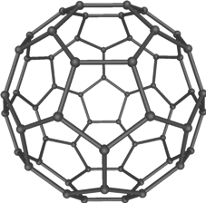
Nevertheless, such calculations are still computationally intense. For example, for a fullerene that contains about 240 carbon atoms, a good quality quantum mechanical calculation  takes more than one minute on about 4,000 Quad-core CPUs (the equivalent of 8 graphics cards like those used in gaming). Such expensive calculation is required to quantitatively understand the unique chemical bonding and reactivity of these extraordinary molecules, which were the subject of the 1996 Chemistry Nobel Prize.   

Although one minute doesn’t sound too long, it is important to realize that to study chemistry, especially in water, we usually have to do each calculation many times.  In molecular dynamics simulations, which are widely used to study processes in solution, one follows the motions of atoms in time to generate a “trajectory.” The trajectory is nothing but a movie for the atoms, from which we can learn about how atoms and molecules interact and react.

Since atoms move rather quickly under room temperature, to track them reliably we have to update their locations after every tiny time increment (called “time step”). How tiny? One femtosecond – that is 10^-15 second! That means that if you wish to use molecular dynamics to follow a process that takes only one microsecond (10^-6 second), you have to perform one billion (10^-6/10^-15=10⁹) calculations! If each calculation takes one minute, that simulation would take 10⁹✕1 min, or about 1900 Years! And that’s only for a “small” molecule that contains merely 240 carbon atoms! The nanoparticles we are interested in easily contain thousands of atoms, and they are surrounded by an even larger number of solvent atoms, ions or other biomolecules. So how can we possibly model things like lipids in a cell membrane, which are still, as Dirac said, “much too complicated to be soluble”?

Clearly, even after tremendous progress in chemistry theory and computing power, it remains a daunting task to generate movies of large molecules or nanoparticles in solution based on quantum mechanics. But what many people don’t know is that Dirac also foresaw this problem, and he actually remarked that:

It therefore becomes desirable that approximate practical methods of applying quantum mechanics should be developed, which can lead to an explanation of the main features of complex atomic systems without too much computation.¹

Remember our shopping cart example? Sometimes a rough estimate can save a lot of time and still get an answer that solves your problem. Coarse-grained models² are one example of Dirac’s “approximate practical methods.” In these models, we make (at least) two major approximations. First, we reduce the resolution of the model. In quantum mechanical models of molecules, we include all the nuclei and electrons, which add up very quickly. In coarse-grained models, we ignore all the electrons and include only the nuclei; in fact, we don’t even include all the nuclei, but group several nuclei together into a single “super atom,” often referred to as a “bead.”

Take water as an example. In a quantum mechanical model, one has to include three nuclei (one oxygen and two hydrogen) and ten electrons (eight from oxygen and one from each hydrogen).

In a popular coarse-grained model called MARTINI (http://cgmartini.nl/), one water bead in fact is meant to represent four water molecules! In the figure below, you can see water beads (A and B) and other examples of coarse-grained models, such as lipids (C), amino acids (E), sugars (D), and fullerene (H).  

The second major approximation we make in coarse-grained models is to simplify the way that beads interact with each other.  Instead of solving for Schrödinger’s equation, which is required in quantum mechanics, we describe the interactions between beads using much simpler equations from classical physics, such as Coulomb’s law. This is possible because our model doesn’t have electrons and therefore the beads are simply spheres with partial charges on them to reflect their distinct chemical nature. For example, a bead representing the phosphate group in a lipid bears negative charge, while a bead representing the amine group in a MTAB ligand on a gold nanoparticle is positively charged.

There are other types of interactions besides charge that we can understand using coarse-grained models as well, but they are all very efficient to compute and orders of magnitude cheaper than any quantum mechanical computations. (In this case “cheaper” means they cost less computing time and energy, which also equals less money in research funding!)

Another consequence of reducing the resolution of the model is that the beads represent groups of atoms and therefore move much slower than individual atoms. As a result, tracking their motions in a molecular dynamics simulation can use much longer time steps. Instead of 1 femtosecond, coarse-grained models like MARTINI often allow the use of 20 to 40 femtoseconds as the time step. 

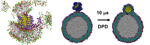
Combining all these benefits together – a much smaller number of beads, much simpler interactions, and longer time steps – coarse-grained molecular dynamics are computationally much more affordable than more complex models. With the MARTINI model, for example, a system that contains a functionalized nanoparticle and a liposome in water, which contains about 0.7 million beads, can be simulated for 25 ns per day using two Graphics Cards! This type of computational efficiency makes it possible to study a broad range of fascinating processes that involve nanoparticles^4,5,6, such as lipid extraction, corona formation (like in the figure above) and even the nanoparticle going inside the membrane of a liposome!

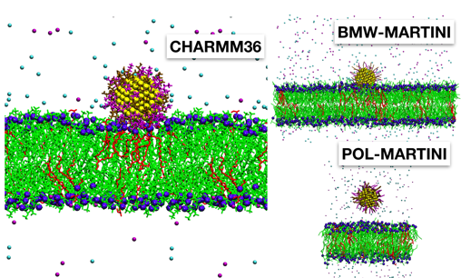
Obviously, such dramatic gain in efficiency is not without its challenges.  Many approximations made in coarse-grained models are rather ad hoc and not straightforward to rationalize. That means that scientists have had to sort of make them up on the spot to find something that worked, but as a result, coarse-grained models can’t always be transferred to new systems.  Therefore, observations from coarse-grained simulations, in the absence of additional data from either experiments or more accurate simulations, are often difficult to evaluate.  One example from our own study⁶ is shown in the figure above: although experimental evidence shows a certain type of nanoparticle sticks to the lipid in the model, one popular variant of the MARTINI model (POL-MARTINI) predicts otherwise. This discrepancy can be traced back to the way that POL-MARTINI describes the behavior of water and ions near the nanoparticle surface.

This is one example of why we always have to be critical of coarse-grained simulations and seek additional data to evaluate the model for each specific system we are interested in. Nevertheless, it is clear that if used properly,^4-7 coarse-grained models are indispensable in understanding the behaviors of nanoparticles in complex chemical and biological environments!

---

---

REFERENCES

1. Dirac, P. Quantum mechanics of many-electron systems, Procedures of the Royal Society of Chemistry, 1929. A 123, No. 792 doi: 10.1098/rspa.1929.0094
2. Voth, Gregory A. Coarse-graining of condensed phase and biomolecular systems. CRC press, 2008. ISBN 9781420059557
3. Marrink, S.J. & Tieleman, D.P. Perspective on the Martini model. Chemical Society Reviews, 2013, 42(16), 6801-6822. doi: 10.1039/C3CS60093A
4. Olenick, L. et al., Lipid Corona Formation from Nanoparticle Interactions with Bilayers, Chem, 2018. 4, 2709-2723.. doi: 10.1016/j.chempr.2018.09.018
5. Chong, G. et al. Defects in Self-Assembled Monolayers on Nanoparticles Prompt Phospholipid Extraction and Bilayer Curvature-Dependent Deformations, Journal of Physical Chemistry C, 2019. 123, 27951-27958. doi: 10.1021/acs.jpcc.9b08583
6. Alipour, E. et al. Phospholipid bilayers: Stability and encapsulation of nanoparticles. Annual Review in Physical Chemistry, 2017. 68, 261-283. doi: 10.1146/annurev-physchem-040215-112634
7. M. Das, et al. Molecular Dynamics Simulation of Interaction between Functionalized Nanoparticles with Lipid Membranes: Analysis of Coarse-grained Models, Journal of Physical Chemistry B, 2019. 123, 10547-104561. doi: 10.1021/acs.jpcb.9b08259